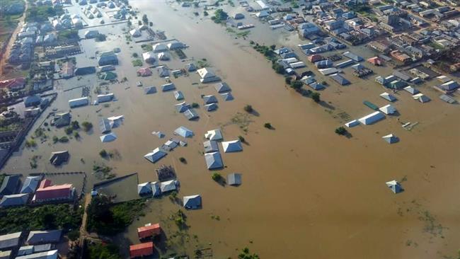
Climate change already impacts the Sahel region with an increase in the occurrence of extreme events such as floods. In Niger, these floods events usually happens along the Niger river. In Niamey, the heavy rains of the end of August and early September resulted in extreme flooding along the river path.
In this post, we will develop a reproducible workflow for a rapid impact assessment of flooding using Sentintel S2 data.
R packages required for the analysis
The following packages will be used for this analysis.
library(tidyverse)
library(sf)
library(stars)
library(sen2r)
library(rhdx) # dickoa/rhdx
library(mapview)
library(units)
library(snapbox)
library(ggthemes) # anthonynorth/snapbox
The packages rhdx and snapbox are not yet on CRAN, you will need the remotes package to get them.
remotes::install_github("dickoa/rhdx")
remotes::install_github("anthonynorth/snapbox")
This analysis is based on a UN-SPIDER tutorial on flood mapping using Sentintel S2 data. In the original article, QGIS was used to map flood extent, here, we are going to do the same analysis using R.
Area of interest
We will restrict this analysis to Niamey and its surrounding where the flood impacted many people lives. The bounding box of the study area can be downloaded here.
bbox_url <- "https://tinyurl.com/yyobbc58"
bbox <- read_sf(bbox_url)
ggplot() +
  layer_mapbox(bbox,
               map_style = mapbox_satellite_streets())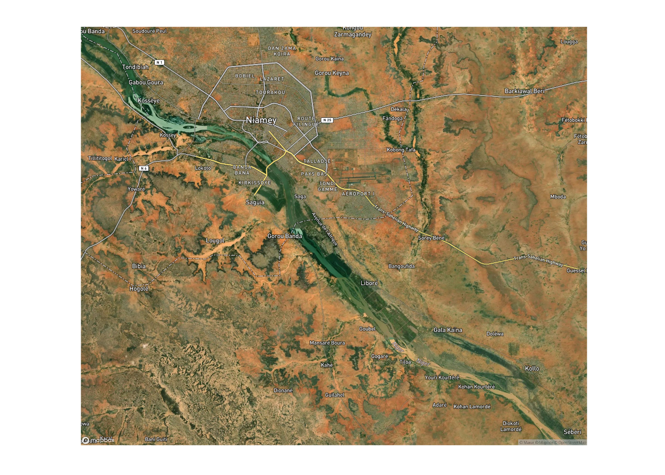
Permanent Water in Niamey
In order to map flood extent, we need to compare the waterbody mapped to a baseline of permanent water. JRC Global Surface Water is an excellent source to access surface water. Permanent water surfaces are defined using the water occurence layer which is the frequency with which water was present in a given pixel from March 1984 to December 2019. Water surfaces are permanent in pixel when it reaches the frequency 100. It means that for this pixel contained water surfaces over the 36 years timespan. In this analysis, the definition is relaxed and permanent water surfaces is defined by water with 80% occurence over 36 years. The data is available online where it can be downloaded.
occurence <- "https://storage.googleapis.com/global-surface-water/downloads2019v2/occurrence/occurrence_0E_20Nv1_1_2019.tif"
occ <- read_stars(occurence) %>%
  st_crop(bbox) %>%
  st_as_stars()
occ
stars object with 2 dimensions and 1 attribute
attribute(s), summary of first 1e+05 cells:
occurrence_0E_20Nv1_1_2019.tif
0 :95865
90 : 324
89 : 299
88 : 268
87 : 151
(Other): 2964
NA's : 129
dimension(s):
from to offset delta refsys point x/y
x 7889 9434 0 0.00025 WGS 84 FALSE [x]
y 25624 26866 20 -0.00025 WGS 84 FALSE [y]Let’s transform the occ raster layer to build build our permanent water layer.
mat <- occ[[1]]
str(mat)
Factor[1:1546, 1:1243] w/ 1783705 levels "0","0","0","0",..: NA 1 1 1 1 1 1 1 1 1 ...
- attr(*, "colors")= chr [1:256] "#FFFFFFFF" "#FEFCFCFF" "#FEF9FAFF" "#FEF7F7FF" ...
- attr(*, "exclude")= logi [1:1783705] FALSE FALSE FALSE FALSE FALSE FALSE ...The data is of factor type, to easily subset the data, we need to convert the type to numeric. Particularly, selecting pixels with an occurence of 80 will be achieved more efficiently with numeric vectors.
mat <- as.numeric(as.character(mat))
mat <- matrix(mat, nrow = dim(occ)[1])
mat[mat < 80] <- NA
mat[!is.na(mat)] <- 1L
occ$water_perm <- mat
occ
stars object with 2 dimensions and 2 attributes
attribute(s), summary of first 1e+05 cells:
occurrence_0E_20Nv1_1_2019.tif water_perm
0 :95865 Min. :1
90 : 324 1st Qu.:1
89 : 299 Median :1
88 : 268 Mean :1
87 : 151 3rd Qu.:1
(Other): 2964 Max. :1
NA's : 129 NA's :98276
dimension(s):
from to offset delta refsys point x/y
x 7889 9434 0 0.00025 WGS 84 FALSE [x]
y 25624 26866 20 -0.00025 WGS 84 FALSE [y]As a final step to have a permanent water layer, the raster layer sais need to turned into a spatial polygon for further analysis. In order to do this transformation, the st_as_sf function can be used to turn it the occ raster to a sf object.
permanent_water <- st_as_sf(occ["water_perm"], merge = TRUE) %>%
  filter(water_perm == 1) %>%
  st_union()

ggplot() +
  layer_mapbox(bbox,
               map_style = mapbox_satellite_streets())  +
  geom_sf(data = permanent_water, fill = "blue", size = 0.2)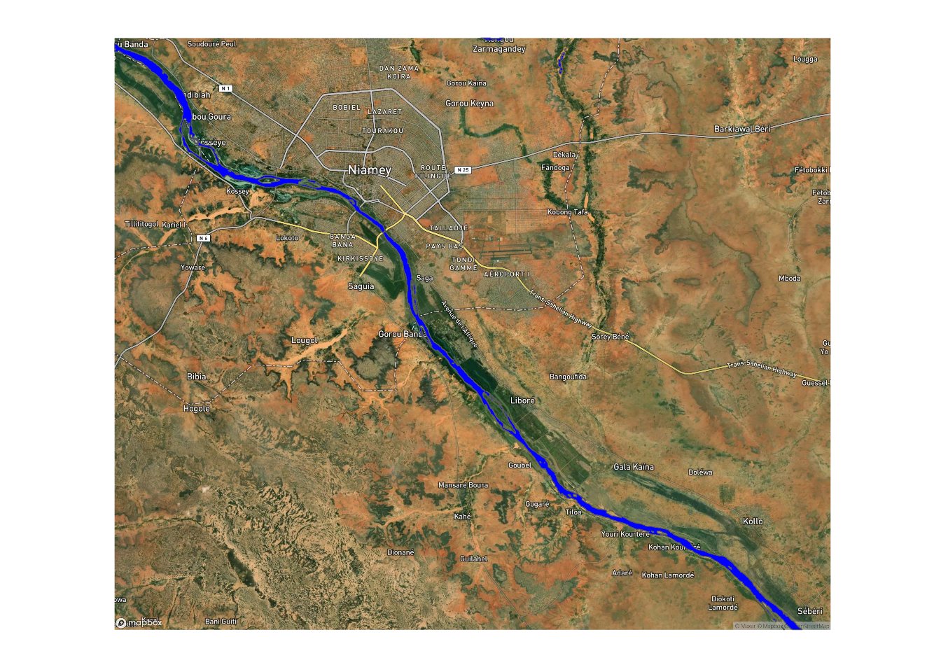
Flood extent using Sentinel S2
A quick survey of the literature suggests that using the Normalized Difference Water Index (NDWI) index allow to easily spot waterbody content. In this analysis, ready to use bottom of atmosphere reflectances products (BOA) will also be used to make it simpler.
It’s defined by the following formulas:
\[NDWI = \dfrac{X_{green} - X_{nir}}{X_{green} + X_{nir}}\]
Where \(X_{green}\) is the green band (B3 at at 842 nm wavelength) and \(X_{nir}\) is the near-infrared (NIR) band (B8, at 842 nm wavelength).
We will use the amazing sen2r R package to download, pre-process and automatically compute the NDWI. In order to download Sentinel S2 data, you will need to register to the Copernicus Open Access Hub and provide your credentials to the sen2r::write_scihub_login function. This analysis will focus on the situation as of September 15th.
write_scihub_login(username = "xxxxx",
                   password = "xxxxx")


out_dir <- "./data/raster/s2out"
safe_dir <- "./data/raster/s2safe"

if (!dir.exists(out_dir))
  dir.create(out_dir, recursive = TRUE)

if (!dir.exists(safe_dir))
  dir.create(safe_dir, recursive = TRUE)

###
out_path <- sen2r(
  gui = FALSE,
  step_atmcorr = "l2a",
  extent = bbox,
  extent_name = "Niamey",
  timewindow = c(as.Date("2020-09-10"), as.Date("2020-09-15")),
  list_prods = "BOA",
  list_indices = "NDWI2",
  list_rgb = "RGB432B",
  path_l1c = safe_dir,
  path_l2a = safe_dir,
  path_out = out_dir,
  parallel = 8,
  overwrite = TRUE
)
There’s two versions of the NDWI index and the one we need is named NDWI2 in the sen2r package.
ndwi <- read_stars(file.path(out_dir,
                             "NDWI2",
                             "S2A2A_20200915_022_Niamey_NDWI2_10.tif"),
                   proxy = FALSE)
ndwi
stars object with 2 dimensions and 1 attribute
attribute(s), summary of first 1e+05 cells:
Min. 1st Qu. Median Mean
S2A2A_20200915_022_Niamey_NDWI... -7223 -4323 -3757 -3673.55
3rd Qu. Max.
S2A2A_20200915_022_Niamey_NDWI... -3067 1271
dimension(s):
from to offset delta refsys point x/y
x 1 4193 388660 10 WGS 84 / UTM zone 31N FALSE [x]
y 1 3450 1503090 -10 WGS 84 / UTM zone 31N FALSE [y]Looking at the ndwi data range, we can rescale the data by dividing by 10000 to simplify the rest of the analysis and map it to visualize this layer.
ndwi[[1]] <- ndwi[[1]]/10000

ggplot() +
  geom_stars(data = ndwi) +
  scale_fill_viridis_c(guide = guide_legend(title = "NDWI",
                                            direction = "horizontal")) +
  theme(legend.position = "bottom")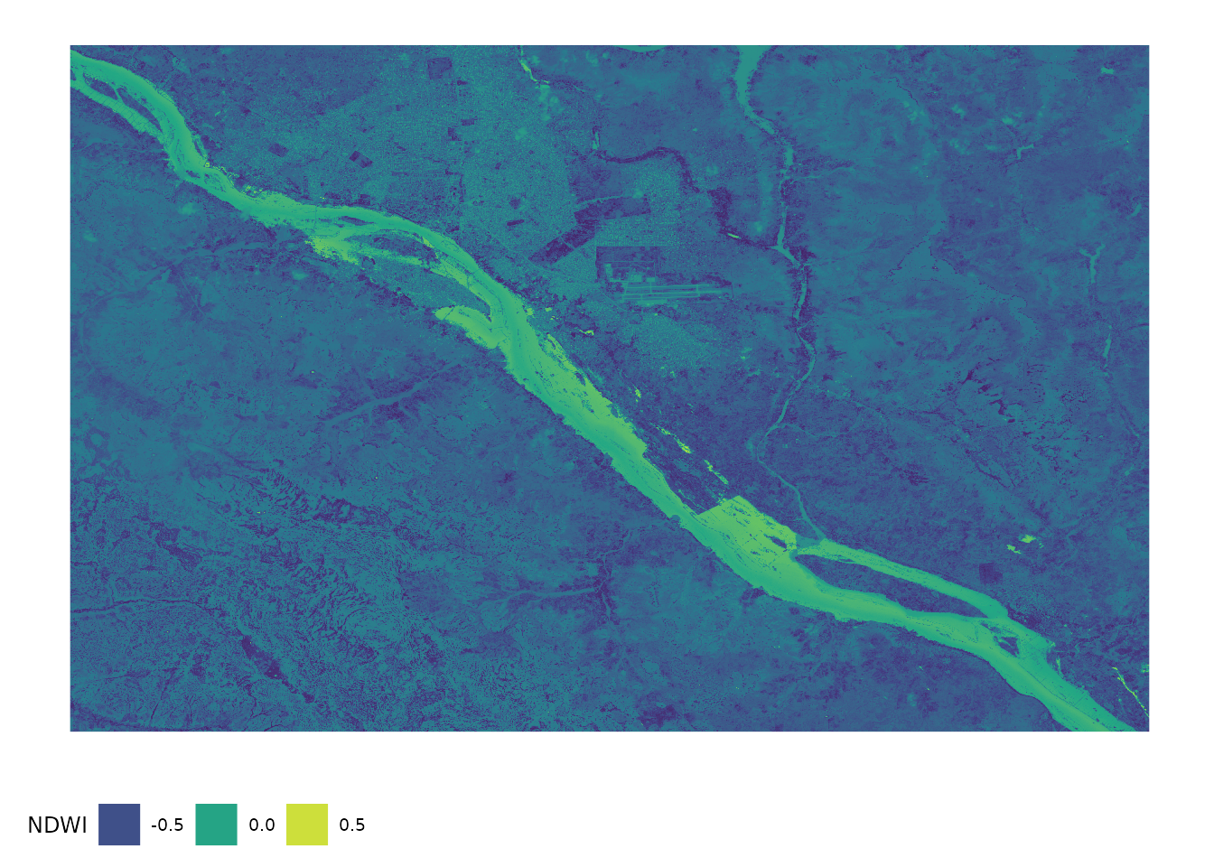
Binarize the NDWI
The next step, is to turn this raster layer into a binary data. The theoretical threshold to select waterbody is set at 0 but we can be more precise and context-specific. We will thus sample NDWI values in pixels we know contains water surface using the permanent_water layer and average these values to get our data.
permanent_water <- st_transform(permanent_water, st_crs(ndwi))
ndwi_water <- st_crop(ndwi,
                      permanent_water)
me <- median(ndwi_water[[1]], na.rm = TRUE)
xbar <- mean(ndwi_water[[1]], na.rm = TRUE)
c(median = me, average = xbar)
median average
0.05250000 0.05067808 All sampled pixels within the permanent water layer can be visualized using an histogram in order its distribution and variability.
hist(ndwi_water[[1]], main = "", xlab = "NDWI")
abline(v = me, col = "red")
abline(v = xbar, col = "blue")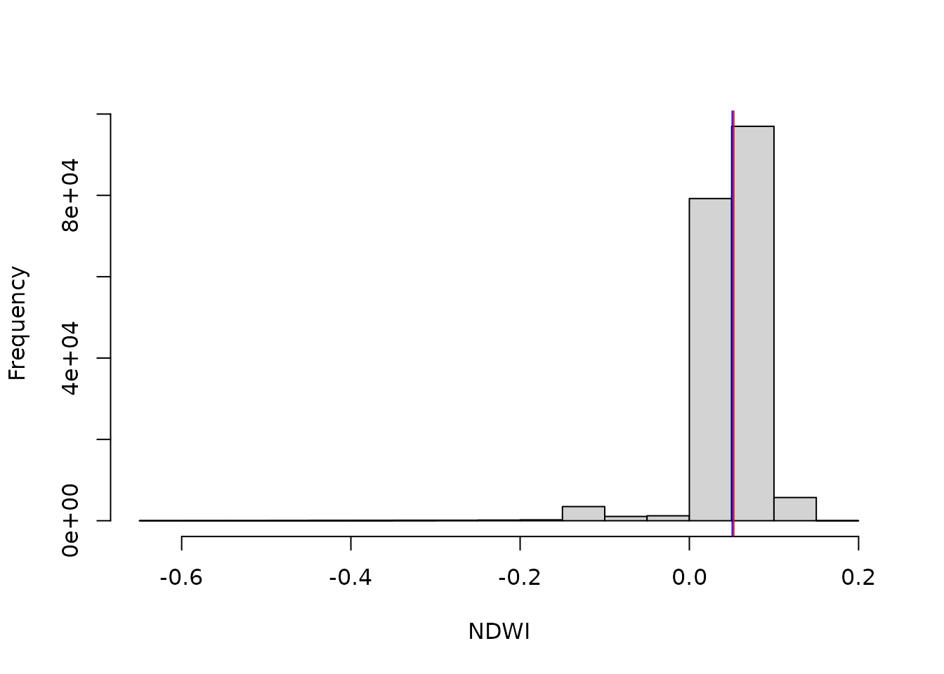
The distribution is unimodal and symmetric around the mode with low variability. Either the average or the median can be used as threshold. For the next step, the median will be used since it’s more robust than the average in general.
ndwi$water_extent <- 1L * (ndwi[[1]] >= me)
ndwi
stars object with 2 dimensions and 2 attributes
attribute(s), summary of first 1e+05 cells:
Min. 1st Qu. Median
S2A2A_20200915_022_Niamey_NDWI... -0.7223 -0.4323 -0.3757
water_extent 0.0000 0.0000 0.0000
Mean 3rd Qu. Max.
S2A2A_20200915_022_Niamey_NDWI... -0.367355 -0.3067 0.1271
water_extent 0.000070 0.0000 1.0000
dimension(s):
from to offset delta refsys point x/y
x 1 4193 388660 10 WGS 84 / UTM zone 31N FALSE [x]
y 1 3450 1503090 -10 WGS 84 / UTM zone 31N FALSE [y]For this data to be used it’s need to be polygonized, we will follow some steps (comments in the code) to make sure the output is good enough for our analysis:
- Polygonize the raster
- Select the polygons containing water surfaces
- Remove polygons smaller than 500 square meters (avoid artificial water bodies, wet rooftops, etc)
- Dissolve and join all polygons into a single polygon
water_extent <- ndwi["water_extent"] %>%
  ## Polygonize the raster
  st_as_sf(merge = TRUE) %>%
  ## select only water extent
  filter(water_extent == 1) %>%
  ## Remove polygons smaller than 500 sqm
  mutate(area = st_area(geometry)) %>% ## compute areas
  filter(area > set_units(500, m^2)) %>%
  ## Dissolve and join all polygons into a single polygon
  st_buffer(dist = set_units(0.5, m)) %>%
  st_union() %>%
  st_simplify(dTolerance = set_units(10, m)) %>%
  st_set_geometry(value = ., x = data.frame(id = 1))

water_extent
Simple feature collection with 1 feature and 1 field
Geometry type: MULTIPOLYGON
Dimension: XY
Bounding box: xmin: 388659.5 ymin: 1468590 xmax: 430590.5 ymax: 1502860
Projected CRS: WGS 84 / UTM zone 31N
id geometry
1 1 MULTIPOLYGON (((430510.2 14...The water_extent derived from NDWI can now be analyzed and visualized.
ggplot() +
  layer_mapbox(bbox,
               map_style = mapbox_satellite_streets())  +
  geom_sf(data = water_extent, fill = "blue", size = 0.2)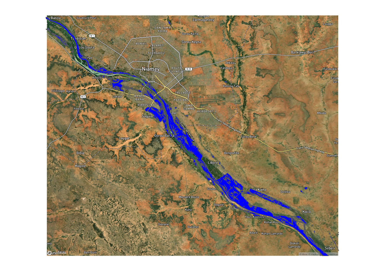
The final step required to obtain the flood extent layer is to remove the permanent water extent (permanent_water) from the waterbody derived from NDWI (water_extent).
flood_extent <- st_difference(water_extent,
                              permanent_water)


ggplot() +
  layer_mapbox(bbox,
               map_style = mapbox_satellite_streets())  +
  geom_sf(data = flood_extent, fill = "blue", size = 0.2)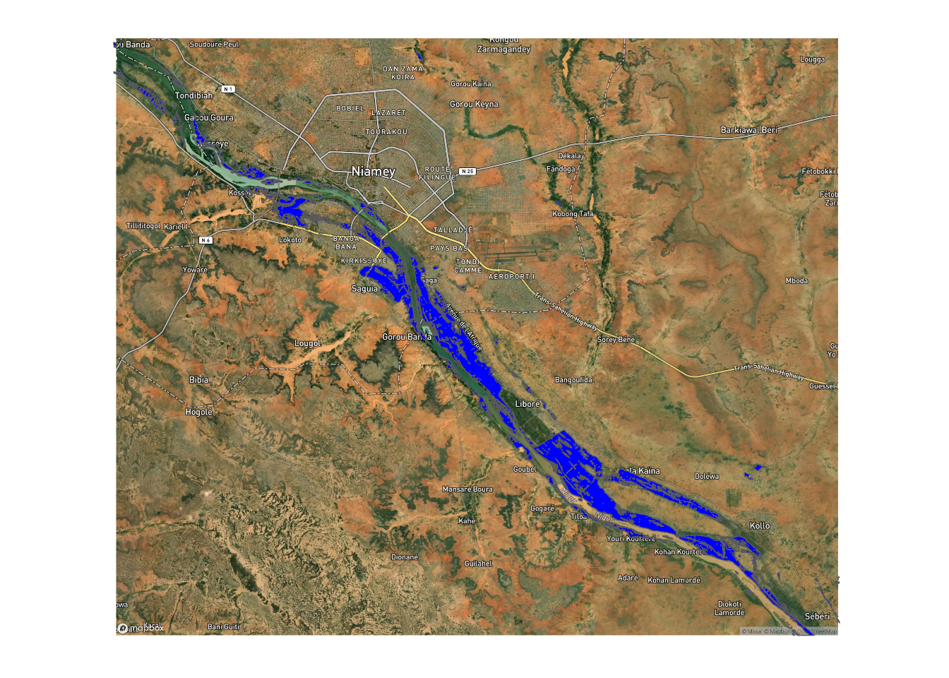
Some statistics can be computed out of the flood_extent and one important metric is the total area of flooded zones within our area of interest.
flood_extent %>%
  st_area() %>%
  set_units(km^2) -> flood_area
flood_area
45.04852 [km^2]45.05 square kilometers of a total area of 1442 square kilometers is flooded as of September 15th.
A second figure of interest is the number of affected buildings. A good source for buildings data is OpenStreetMap (OSM) and Niger has one vibrant OSM community, so the data is of good quality particularly in cities like Niamey. Once again, the data is available on HDX.
ner_bu <- pull_dataset("hotosm_niger_buildings") %>%
  get_resource(1) %>%
  read_resource()

ner_bu <- st_transform(ner_bu, st_crs(flood_extent))

ner_bu <- st_crop(ner_bu, flood_extent)
ner_bu_centroid <- st_point_on_surface(ner_bu)

impacted_bu <- st_intersection(ner_bu_centroid, flood_extent)
We estimated around 421 potentially affected building in the study area.
Limitations
The goal of this analysis was to show how to conduct a reproducible rapid flood mapping and damage assessment using R and Sentintel S2 data. We made several choices during the process and they all have an impact on the final results. For example, other spectral indices could have been used, some authors suggested that Modified NDWI (MDNWI) is more accurate in urban settings and others advocated for the use the Normalized Difference Flood Index for this type of analysis (NDFI). The package sen2r is quite flexible and allow to easily add all the above indices. Finally, SAR imagery can also be used to push the analysis further and estimate for example indicators such as flood water depth for better planing of a response plan.
Session info for this analysis.
Session info
devtools::session_info()─ Session info ────────────────────────────────────────────────
setting value
version R version 4.2.2 Patched (2022-11-12 r83340)
os Arch Linux
system x86_64, linux-gnu
ui X11
language en_US.UTF-8
collate en_US.UTF-8
ctype en_US.UTF-8
tz UTC
date 2022-12-28
pandoc 2.19.2 @ /usr/bin/ (via rmarkdown)
─ Packages ────────────────────────────────────────────────────
package * version date (UTC) lib source
abind * 1.4-5 2016-07-21 [1] CRAN (R 4.2.2)
assertthat 0.2.1 2019-03-21 [1] CRAN (R 4.2.2)
backports 1.4.1 2021-12-13 [1] CRAN (R 4.2.2)
base64enc 0.1-3 2015-07-28 [1] CRAN (R 4.2.2)
broom 1.0.2 2022-12-15 [1] CRAN (R 4.2.2)
cachem 1.0.6 2021-08-19 [1] CRAN (R 4.2.2)
callr 3.7.3 2022-11-02 [1] CRAN (R 4.2.2)
cellranger 1.1.0 2016-07-27 [1] CRAN (R 4.2.2)
class 7.3-20 2022-01-16 [1] CRAN (R 4.2.2)
classInt 0.4-8 2022-09-29 [1] CRAN (R 4.2.2)
cli 3.5.0 2022-12-20 [1] CRAN (R 4.2.2)
codetools 0.2-18 2020-11-04 [1] CRAN (R 4.2.2)
colorspace 2.0-3 2022-02-21 [1] CRAN (R 4.2.2)
crayon 1.5.2 2022-09-29 [1] CRAN (R 4.2.2)
crosstalk 1.2.0 2021-11-04 [1] CRAN (R 4.2.2)
crul 1.3 2022-09-03 [1] CRAN (R 4.2.2)
curl 4.3.3 2022-10-06 [1] CRAN (R 4.2.2)
data.table 1.14.6 2022-11-16 [1] CRAN (R 4.2.2)
DBI 1.1.3 2022-06-18 [1] CRAN (R 4.2.2)
dbplyr 2.2.1 2022-06-27 [1] CRAN (R 4.2.2)
devtools 2.4.5 2022-10-11 [1] CRAN (R 4.2.2)
digest 0.6.31 2022-12-11 [1] CRAN (R 4.2.2)
doParallel 1.0.17 2022-02-07 [1] CRAN (R 4.2.2)
dplyr * 1.0.10 2022-09-01 [1] CRAN (R 4.2.2)
e1071 1.7-12 2022-10-24 [1] CRAN (R 4.2.2)
ellipsis 0.3.2 2021-04-29 [1] CRAN (R 4.2.2)
evaluate 0.19 2022-12-13 [1] CRAN (R 4.2.2)
fansi 1.0.3 2022-03-24 [1] CRAN (R 4.2.2)
fastmap 1.1.0 2021-01-25 [1] CRAN (R 4.2.2)
forcats * 0.5.2 2022-08-19 [1] CRAN (R 4.2.2)
foreach 1.5.2 2022-02-02 [1] CRAN (R 4.2.2)
foreign 0.8-84 2022-12-06 [1] CRAN (R 4.2.2)
fs 1.5.2 2021-12-08 [1] CRAN (R 4.2.2)
gargle 1.2.1 2022-09-08 [1] CRAN (R 4.2.2)
generics 0.1.3 2022-07-05 [1] CRAN (R 4.2.2)
geojson 0.3.4 2020-06-23 [1] CRAN (R 4.2.2)
geojsonio 0.10.0 2022-10-07 [1] CRAN (R 4.2.2)
geojsonsf 2.0.3 2022-05-30 [1] CRAN (R 4.2.2)
ggplot2 * 3.4.0 2022-11-04 [1] CRAN (R 4.2.2)
ggthemes * 4.2.4 2021-01-20 [1] CRAN (R 4.2.2)
glue 1.6.2 2022-02-24 [1] CRAN (R 4.2.2)
googledrive 2.0.0 2021-07-08 [1] CRAN (R 4.2.2)
googlesheets4 1.0.1 2022-08-13 [1] CRAN (R 4.2.2)
gtable 0.3.1 2022-09-01 [1] CRAN (R 4.2.2)
haven 2.5.1 2022-08-22 [1] CRAN (R 4.2.2)
hms 1.1.2 2022-08-19 [1] CRAN (R 4.2.2)
hoardr 0.5.2 2018-12-02 [1] CRAN (R 4.2.2)
htmltools 0.5.4 2022-12-07 [1] CRAN (R 4.2.2)
htmlwidgets 1.6.0 2022-12-15 [1] CRAN (R 4.2.2)
httpcode 0.3.0 2020-04-10 [1] CRAN (R 4.2.2)
httpuv 1.6.7 2022-12-14 [1] CRAN (R 4.2.2)
httr 1.4.4 2022-08-17 [1] CRAN (R 4.2.2)
iterators 1.0.14 2022-02-05 [1] CRAN (R 4.2.2)
jqr 1.2.3 2022-03-10 [1] CRAN (R 4.2.2)
jsonlite 1.8.4 2022-12-06 [1] CRAN (R 4.2.2)
KernSmooth 2.23-20 2021-05-03 [1] CRAN (R 4.2.2)
knitr 1.41 2022-11-18 [1] CRAN (R 4.2.2)
later 1.3.0 2021-08-18 [1] CRAN (R 4.2.2)
lattice 0.20-45 2021-09-22 [1] CRAN (R 4.2.2)
lazyeval 0.2.2 2019-03-15 [1] CRAN (R 4.2.2)
leafem 0.2.0 2022-04-16 [1] CRAN (R 4.2.2)
leaflet 2.1.1 2022-03-23 [1] CRAN (R 4.2.2)
lifecycle 1.0.3 2022-10-07 [1] CRAN (R 4.2.2)
lubridate 1.9.0 2022-11-06 [1] CRAN (R 4.2.2)
lwgeom 0.2-10 2022-11-19 [1] CRAN (R 4.2.2)
magrittr 2.0.3 2022-03-30 [1] CRAN (R 4.2.2)
maptools 1.1-6 2022-12-14 [1] CRAN (R 4.2.2)
mapview * 2.11.0 2022-04-16 [1] CRAN (R 4.2.2)
memoise 2.0.1 2021-11-26 [1] CRAN (R 4.2.2)
mime 0.12 2021-09-28 [1] CRAN (R 4.2.2)
miniUI 0.1.1.1 2018-05-18 [1] CRAN (R 4.2.2)
modelr 0.1.10 2022-11-11 [1] CRAN (R 4.2.2)
munsell 0.5.0 2018-06-12 [1] CRAN (R 4.2.2)
pillar 1.8.1 2022-08-19 [1] CRAN (R 4.2.2)
pkgbuild 1.4.0 2022-11-27 [1] CRAN (R 4.2.2)
pkgconfig 2.0.3 2019-09-22 [1] CRAN (R 4.2.2)
pkgload 1.3.2 2022-11-16 [1] CRAN (R 4.2.2)
png 0.1-8 2022-11-29 [1] CRAN (R 4.2.2)
prettyunits 1.1.1 2020-01-24 [1] CRAN (R 4.2.2)
processx 3.8.0 2022-10-26 [1] CRAN (R 4.2.2)
profvis 0.3.7 2020-11-02 [1] CRAN (R 4.2.2)
promises 1.2.0.1 2021-02-11 [1] CRAN (R 4.2.2)
proxy 0.4-27 2022-06-09 [1] CRAN (R 4.2.2)
ps 1.7.2 2022-10-26 [1] CRAN (R 4.2.2)
purrr * 1.0.0 2022-12-20 [1] CRAN (R 4.2.2)
R6 2.5.1 2021-08-19 [1] CRAN (R 4.2.2)
ragg 1.2.4 2022-10-24 [1] CRAN (R 4.2.2)
rappdirs 0.3.3 2021-01-31 [1] CRAN (R 4.2.2)
raster 3.6-11 2022-11-28 [1] CRAN (R 4.2.2)
Rcpp 1.0.9 2022-07-08 [1] CRAN (R 4.2.2)
RcppTOML 0.1.7 2020-12-02 [1] CRAN (R 4.2.2)
readr * 2.1.3 2022-10-01 [1] CRAN (R 4.2.2)
readxl 1.4.1 2022-08-17 [1] CRAN (R 4.2.2)
remotes 2.4.2 2021-11-30 [1] CRAN (R 4.2.2)
reprex 2.0.2 2022-08-17 [1] CRAN (R 4.2.2)
rgdal 1.6-3 2022-12-14 [1] CRAN (R 4.2.2)
rgeos 0.6-1 2022-12-14 [1] CRAN (R 4.2.2)
rhdx * 0.1.0.9000 2022-11-03 [1] gitlab (dickoa/rhdx@c443336)
rlang 1.0.6 2022-09-24 [1] CRAN (R 4.2.2)
rmarkdown 2.19 2022-12-15 [1] CRAN (R 4.2.2)
rvest 1.0.3 2022-08-19 [1] CRAN (R 4.2.2)
s2 1.1.1 2022-11-17 [1] CRAN (R 4.2.2)
satellite 1.0.4 2021-10-12 [1] CRAN (R 4.2.2)
scales 1.2.1 2022-08-20 [1] CRAN (R 4.2.2)
sen2r * 1.5.3 2022-09-22 [1] CRAN (R 4.2.2)
sessioninfo 1.2.2 2021-12-06 [1] CRAN (R 4.2.2)
sf * 1.0-9 2022-11-08 [1] CRAN (R 4.2.2)
shiny 1.7.4 2022-12-15 [1] CRAN (R 4.2.2)
snapbox * 0.2.2 2022-12-28 [1] Github (anthonynorth/snapbox@f7d05d2)
sp 1.5-1 2022-11-07 [1] CRAN (R 4.2.2)
stars * 0.6-0 2022-11-21 [1] CRAN (R 4.2.2)
stringi 1.7.8 2022-07-11 [1] CRAN (R 4.2.2)
stringr * 1.5.0 2022-12-02 [1] CRAN (R 4.2.2)
stylebox 0.3.0 2022-12-28 [1] Github (anthonynorth/stylebox@be15f46)
systemfonts 1.0.4 2022-02-11 [1] CRAN (R 4.2.2)
terra 1.6-47 2022-12-02 [1] CRAN (R 4.2.2)
textshaping 0.3.6 2021-10-13 [1] CRAN (R 4.2.2)
tibble * 3.1.8 2022-07-22 [1] CRAN (R 4.2.2)
tidyr * 1.2.1 2022-09-08 [1] CRAN (R 4.2.2)
tidyselect 1.2.0 2022-10-10 [1] CRAN (R 4.2.2)
tidyverse * 1.3.2 2022-07-18 [1] CRAN (R 4.2.2)
timechange 0.1.1 2022-11-04 [1] CRAN (R 4.2.2)
tzdb 0.3.0 2022-03-28 [1] CRAN (R 4.2.2)
units * 0.8-1 2022-12-10 [1] CRAN (R 4.2.2)
urlchecker 1.0.1 2021-11-30 [1] CRAN (R 4.2.2)
usethis 2.1.6 2022-05-25 [1] CRAN (R 4.2.2)
utf8 1.2.2 2021-07-24 [1] CRAN (R 4.2.2)
V8 4.2.2 2022-11-03 [1] CRAN (R 4.2.2)
vctrs 0.5.1 2022-11-16 [1] CRAN (R 4.2.2)
webshot 0.5.4 2022-09-26 [1] CRAN (R 4.2.2)
withr 2.5.0 2022-03-03 [1] CRAN (R 4.2.2)
wk 0.7.1 2022-12-09 [1] CRAN (R 4.2.2)
xfun 0.36 2022-12-21 [1] CRAN (R 4.2.2)
XML 3.99-0.13 2022-12-04 [1] CRAN (R 4.2.2)
xml2 1.3.3 2021-11-30 [1] CRAN (R 4.2.2)
xtable 1.8-4 2019-04-21 [1] CRAN (R 4.2.2)
yaml 2.3.6 2022-10-18 [1] CRAN (R 4.2.2)
[1] /usr/lib/R/library
───────────────────────────────────────────────────────────────