3  Stratification and sample allocation

Stratification divides the population before sampling. An allocation then decides how many units to select from each stratum. A domain is different. It is a population for which an estimate is required, and it can contain one or more strata.

This chapter covers allocation for one indicator. Chapter 2 combines several requirements into one total, and Chapter 4 finds one allocation that satisfies several estimands and domains simultaneously.

3.1 Allocate a fixed sample

The frame has one row per stratum. N is the population size, sd is the anticipated within-stratum standard deviation, and mean supplies the scale for a CV calculation:

frame <- data.frame(
  stratum = c("Urban", "Peri-urban", "Rural"),
  N = c(4000, 3000, 3000),
  sd = c(10, 15, 8),
  mean = c(50, 60, 55)
)

allocation <- n_alloc(frame, n = 600, alloc = "neyman")
allocation
#> Stratum allocation (neyman, 3 strata)
#> field design: n = 600, cv = 0.0079, cost = 600
#> continuous optimum: n = 600, cv = 0.0079, se = 0.4305
#> (deff = 1)
#> design df = 597

Neyman allocation places more sample where \(N_hS_h\) is larger. The result keeps a continuous optimum in $detail$n and a whole-unit fieldwork proposal in $detail$n_int:

allocation$detail[, c("stratum", "N", "n", "n_int", "weight")]
#>      stratum    N        n n_int   weight
#> 1      Urban 4000 220.1835   220 18.16667
#> 2 Peri-urban 3000 247.7064   248 12.11111
#> 3      Rural 3000 132.1101   132 22.70833

Use the operational column when issuing a sample. Its planned weight is the population-to-sample ratio for the allocation, not a final analysis weight adjusted for realized selection and response.

3.2 Check an operational allocation

prec_alloc() evaluates any proposed set of stratum sample sizes. Passing the planning result evaluates its continuous design. Supply the integer column to check the whole-unit fieldwork design:

prec_alloc(allocation)
#> Sampling precision for alloc
#> n = 600 (3 strata)
#> se = 0.4305, moe = 0.8438, cv = 0.0079, rmoe = 0.0155
prec_alloc(allocation, n = allocation$detail$n_int)
#> Sampling precision for alloc
#> n = 600 (3 strata)
#> se = 0.4305, moe = 0.8438, cv = 0.0079, rmoe = 0.0155

The detail table shows how much each stratum contributes to overall variance. .share sums to 1:

assessment <- prec_alloc(allocation, n = allocation$detail$n_int)
assessment$detail[, c("stratum", "n", ".se", ".cv", ".share")]
#>      stratum   n       .se        .cv    .share
#> 1      Urban 220 0.6553972 0.01310794 0.3708035
#> 2 Peri-urban 248 0.9122818 0.01520470 0.4041246
#> 3      Rural 132 0.6808195 0.01237854 0.2250719

3.3 Solve for precision or budget

Instead of fixing total n, ask for a target CV:

n_alloc(frame, cv = 0.04, alloc = "neyman")
#> Stratum allocation (neyman, 3 strata)
#> field design: n = 27, cv = 0.0384, cost = 27
#> continuous optimum: n = 24.93353, cv = 0.0400, se = 2.1800
#> (deff = 1)
#> design df = 24

For budget allocation, add a cost per sampled unit and use the optimal cost-adjusted rule:

cost_frame <- transform(frame, unit_cost = c(1, 1.5, 2.5))
n_alloc(cost_frame, budget = 900, alloc = "optimal")
#> Stratum allocation (optimal, 3 strata)
#> field design: n = 621, cv = 0.0079, cost = 900
#> continuous optimum: n = 621.7392, cv = 0.0079, se = 0.4290
#> (deff = 1)
#> design df = 618

The three common rules answer different questions:

Rule	Relative allocation	Use
"proportional"	\(N_h\)	Equal sampling fractions.
"neyman"	\(N_hS_h\)	Minimize variance with equal unit costs.
"optimal"	\(N_hS_h/\sqrt{c_h}\)	Minimize variance with unequal unit costs.

alloc = "power" implements Bankier allocation (Bankier 1988), with weights proportional to the population CV sd / abs(mean) times alloc_measure^alloc_q. The allocation measure defaults to N * abs(mean), and with that default alloc_q = 1 gives Neyman allocation. At alloc_q = 0 the weights are the population CVs whatever the measure. Means must be nonzero. The population CV describes variation among units and differs from the cv precision target, which describes the relative standard error of an estimate.

Supply a positive alloc_measure column to use another stratum measure:

bankier_frame <- transform(frame, alloc_measure = N)
n_alloc(bankier_frame, n = 600, alloc = "power", alloc_q = 0.5)
#> Stratum allocation (power, 3 strata)
#> field design: n = 600, cv = 0.0079, cost = 600
#> continuous optimum: n = 600, cv = 0.0079, se = 0.4308
#> (deff = 1)
#> design df = 597

With a custom measure, alloc_q = 1 need not give Neyman allocation. Stratum-specific response rates and design effects multiply the weights by sqrt(deff / resp_rate). Bankier allocation does not generally equalize domain CVs. Use explicit domain targets when comparable precision is required.

3.4 Add operational constraints

Minimum stratum sizes, maximum planned weights, and census strata can be declared with min_n_stratum, max_weight, and take_all:

constrained_frame <- transform(
  frame,
  unit_cost = c(1, 1.5, 1),
  max_weight = c(25, 20, NA),
  take_all = c(FALSE, FALSE, TRUE)
)

constrained <- n_alloc(
  constrained_frame,
  budget = 3500,
  alloc = "optimal",
  min_n_stratum = 40
)
constrained
#> Stratum allocation (optimal, 3 strata)
#> field design: n = 3403, cv = 0.0076, cost = 3500
#> continuous optimum: n = 3403.425, cv = 0.0076, se = 0.4125
#> (min_n_stratum = 40, deff = 1)
#> design df = 401

The constraints change the optimum, so assess the returned operational design as a unit. Independently rounding continuous stratum values can violate a budget or precision requirement.

3.4.1 Fieldwork assumptions by stratum

deff and resp_rate can be scalar values or frame columns. Stratum-specific response rates change both the number issued and the best allocation:

response_frame <- transform(
  frame,
  resp_rate = c(0.92, 0.80, 0.65)
)

response_plan <- n_alloc(response_frame, n = 600, alloc = "neyman")
response_plan$detail[, c("stratum", "n", "n_int")]
#>      stratum        n n_int
#> 1      Urban 205.4620   205
#> 2 Peri-urban 247.8752   248
#> 3      Rural 146.6628   147

The response adjustment sets an expected responding count. It does not remove nonresponse bias. Use the two-phase methods of Chapter 6 when a subsample of nonrespondents will receive additional follow-up.

3.5 Require precision for domains

When each domain is a union of complete strata, domains requests a target for every domain:

domain_frame <- data.frame(
  province = c("North", "North", "South", "South"),
  stratum = c("Urban", "Rural", "Urban", "Rural"),
  N = c(2000, 3000, 1800, 3200),
  sd = c(12, 18, 10, 16),
  mean = c(55, 48, 58, 50)
)

domain_plan <- n_alloc(
  domain_frame,
  domains = "province",
  cv = 0.04,
  alloc = "power",
  alloc_q = 0.3
)
domain_plan
#> Stratum allocation (power, 4 strata)
#> field design: n = 110, cv = 0.0271, cost = 110
#> continuous optimum: n = 108.2371, cv = 0.0273, se = 1.4160
#> (deff = 1)
#> design df = 106
#> Domains: 2
#> 
#>  province .domain .n       .se     .moe     .rmoe      .cv   
#>  North    5_North 58.67031 2.03200 3.982647 0.07839856 0.0400
#>  South    5_South 49.56679 1.97265 3.866324 0.07311505 0.0373
#>  .cost
#>  59   
#>  50
domain_plan$domains
#>   province .domain       .n     .se     .moe      .rmoe
#> 1    North 5_North 58.67031 2.03200 3.982647 0.07839856
#> 2    South 5_South 49.56679 1.97265 3.866324 0.07311505
#>          .cv    .cost
#> 1 0.04000000 58.67031
#> 2 0.03730428 49.56679

These domains are known on the frame. For a domain that appears naturally within one sample and is not identified on the frame, size the sample from the domain’s expected share, as described in Chapter 2. That calculation applies to single-stage indicator tables only, because a population share alone does not describe how domain members spread across clusters.

3.6 Construct candidate strata

When a continuous auxiliary variable is available on the frame, strata_bound() constructs candidate boundaries. The objective is the precision of the auxiliary variable itself, so its usefulness for a study variable depends on how closely the two are related.

set.seed(12345)
x <- rlnorm(5000, meanlog = 6, sdlog = 1.2)

boundaries <- strata_bound(
  x,
  n_strata = 4,
  cv = 0.05,
  method = "cumrootf"
)
boundaries
#> Strata boundaries (Dalenius-Hodges, 4 strata)
#> n = 63, cv = 0.0491, allocation: neyman
#> 
#>  stratum  lower upper    N share     sd   mean  n
#>        1 3.8267   400 2473 0.495  105.3  191.4 10
#>        2    400  1200 1647 0.329  222.7  700.6 14
#>        3   1200  3100  672 0.134  519.5 1871.7 14
#>        4   3100 21958  208 0.042 3094.3 5543.6 25

Four methods are available:

Method	Character
"cumrootf"	Fast Dalenius–Hodges cumulative root frequency rule.
"geo"	Fast geometric progression, useful for skewed values.
"lh"	LH-inspired coordinate search.
"kozak"	Kozak random search, exact by enumeration on small problems.

The last two are heuristics. Their results are candidates rather than certified global optima.

The Kozak search starts from more points than the LH search, so it costs more run time, but more starting points do not guarantee a better partition. At a fixed sample size, compare the CV each method reaches on the frame at hand:

set.seed(2024)
kozak_boundaries <- strata_bound(x, n_strata = 4, n = 300, method = "kozak")
kozak_boundaries
#> Strata boundaries (Kozak random search, 4 strata, converged)
#> n = 300, cv = 0.0195, allocation: neyman
#> 
#>  stratum  lower  upper    N share     sd   mean   n
#>        1 3.8267 490.12 2835 0.567  129.7  223.6  70
#>        2 490.12 1356.2 1406 0.281  236.4  816.2  63
#>        3 1356.2 3571.6  596 0.119  579.7 2101.8  66
#>        4 3571.6  21958  163 0.033 3234.5 6160.1 101

method_cv <- c(
  sapply(c("cumrootf", "geo", "lh"), function(method) {
    strata_bound(x, n_strata = 4, n = 300, method = method)$cv
  }),
  kozak = kozak_boundaries$cv
)
round(method_cv, 4)
#> cumrootf      geo       lh    kozak 
#>   0.0199   0.0320   0.0195   0.0195

On this variable the LH and Kozak searches reach the same smallest CV, the cumulative root frequency rule comes close, and the geometric rule falls well behind.

The search allocates each candidate partition by Neyman allocation unless alloc says otherwise. With alloc = "power", it uses the Bankier rule (Bankier 1988)

\[ n_h \propto \frac{S_h}{|\bar{X}_h|}\left(N_h|\bar{X}_h|\right)^q, \]

where \(S_h\) and \(\bar{X}_h\) are the standard deviation and mean of x in stratum \(h\), \(N_h\) is the stratum population, and \(q\) is alloc_q. The population CV \(S_h/|\bar{X}_h|\) and the measure \(N_h|\bar{X}_h|\) are recomputed for every candidate partition, so the allocation rule shapes the cut points:

strata_bound(x, n_strata = 4, n = 300, alloc = "power", alloc_q = 0.5)
#> Strata boundaries (LH-inspired coordinate search, 4 strata, converged)
#> n = 300, cv = 0.0197, allocation: power (alloc_q = 0.50)
#> 
#>  stratum  lower  upper    N share     sd   mean  n
#>        1 3.8267 510.33 2893 0.579  134.2  229.1 89
#>        2 510.33 1378.7 1361 0.272  236.8  834.9 57
#>        3 1378.7 3571.6  583 0.117  575.6 2118.1 56
#>        4 3571.6  21958  163 0.033 3234.5 6160.1 98

At alloc_q = 1 the rule is Neyman allocation. At alloc_q = 0 the sample is proportional to the stratum population CVs. The rule does not generally equalize stratum CVs. Because it divides by each stratum mean, x should be a positive size measure. To use an allocation measure other than \(N_h|\bar{X}_h|\), construct the strata first and then add an alloc_measure column to the frame passed to n_alloc().

predict() applies the learned boundaries to new observations:

predict(
  boundaries,
  newdata = c(100, 500, 1500, 5000),
  labels = paste0("S", 1:4)
)
#> [1] S1 S2 S3 S4
#> Levels: S1 S2 S3 S4

The strata table connects directly to n_alloc():

allocated_boundaries <- n_alloc(boundaries$strata, cv = 0.05)
allocated_boundaries
#> Stratum allocation (neyman, 4 strata)
#> field design: n = 63, cv = 0.0491, cost = 63
#> continuous optimum: n = 60.95014, cv = 0.0500, se = 40.3814
#> (deff = 1)
#> design df = 59

Both functions use the same variance calculation. Design assumptions carry through both, passed directly or through a svyplan() profile:

plan <- svyplan(deff = 1.8, resp_rate = 0.85)
planned_boundaries <- strata_bound(x, n_strata = 4, cv = 0.05, plan = plan)
c(
  strata_bound = planned_boundaries$n,
  n_alloc = n_alloc(planned_boundaries$strata, cv = 0.05, plan = plan)$n
)
#> strata_bound      n_alloc 
#>     118.0000     116.4124

The difference between the two totals is whole-unit rounding, not a change of model. strata_bound() reports the whole-unit allocation in $strata$n, whereas n_alloc() reports the continuous optimum.

A scalar deff does not move the cut points. At a fixed sample size it multiplies the variance of every candidate partition by the same factor, so the same partition remains best and only the reported CV changes:

rbind(
  deff_1.0 = strata_bound(x, n_strata = 4, n = 300)$boundaries,
  deff_1.8 = strata_bound(x, n_strata = 4, n = 300, deff = 1.8)$boundaries
)
#>              [,1]     [,2]    [,3]
#> deff_1.0 490.1171 1356.216 3571.62
#> deff_1.8 490.1171 1356.216 3571.62

Under a cv target, what deff changes is the n the target requires.

Compare the stratum sampling fractions before deciding whether the proposed boundaries create workable fieldwork loads:

plot(boundaries)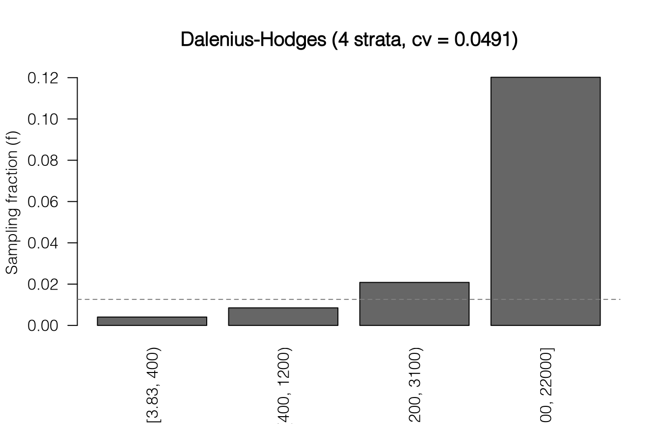

Sampling fractions under the candidate four-stratum design. Compare each stratum with the dashed overall fraction to identify where sampling is most intensive.

3.7 Draw an allocation and map it

An allocation becomes a sample once a design selects units under it. Here the strata are the 13 regions of Burkina Faso and the units are the EAs of bfa_eas. The n_alloc() frame counts EAs per region and takes the prior standard deviation and the cost per visited EA from bfa_eas_variance and bfa_eas_cost, both synthetic teaching inputs.

region_strata <- bfa_eas |>
  count(stratum = region, name = "N") |>
  left_join(rename(bfa_eas_variance, stratum = region), by = "stratum") |>
  left_join(rename(bfa_eas_cost, stratum = region), by = "stratum") |>
  mutate(sd = sqrt(var), unit_cost = cost, .keep = "unused")

region_allocations <- list(
  Proportional = n_alloc(region_strata, n = 300, alloc = "proportional"),
  `Optimal, at least 20 per region` =
    n_alloc(region_strata, n = 300, alloc = "optimal", min_n_stratum = 20)
)

The cost-adjusted rule alone would move only a few EAs, because the regional standard deviations are close and the square roots of the costs differ by less than 40 percent. The floor of 20 EAs per region matters more. It gives every region a sample large enough for its own estimate, and the national standard error pays for it:

sapply(region_allocations, \(a) prec_alloc(a, n = a$detail$n_int)$se)
#>                    Proportional Optimal, at least 20 per region 
#>                      0.03513676                      0.03602163

samplyr takes the whole-unit allocation as a table keyed by the stratification variable:

region_samples <- lapply(region_allocations, \(a) {
  takes <- data.frame(region = a$detail$stratum, n = a$detail$n_int)
  sampling_design() |>
    stratify_by(region) |>
    draw(n = takes) |>
    execute(bfa_eas, seed = 7)
})

allocation_names <- names(region_allocations)

selected <- bind_rows(lapply(region_samples, as.data.frame),
                      .id = "allocation") |>
  mutate(allocation = factor(allocation, allocation_names))

rates <- bind_rows(lapply(region_allocations, \(a) a$detail),
                   .id = "allocation") |>
  transmute(allocation = factor(allocation, allocation_names),
            region = stratum,
            `EAs per 1,000` = 1000 * n_int / N)

map_eas(selected, facet = "allocation",
        fill_data = rates, fill = "EAs per 1,000")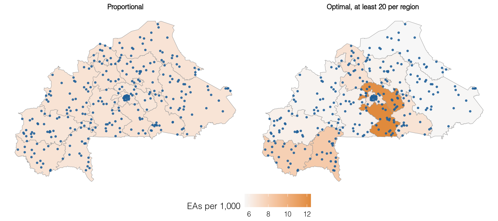

The same 300 EAs under two allocations. Shading is the regional sampling rate and each point is a selected EA.

Under proportional allocation every region is sampled at the same rate, so the points simply follow where EAs are dense. The floor lifts the four smallest regions, Cascades, Centre-Sud, Plateau-Central and Sud-Ouest, and the large regions such as Est and Boucle du Mouhoun give up EAs to pay for them. Those differences in sampling rate are the differences in design weight that an analysis of the national sample must carry.

3.8 Beyond one indicator

Several later designs build on this single-indicator allocation. Chapter 2 explains how indicator requirements combine, including separate quotas and naturally occurring domains. Chapter 4 satisfies several indicator and overlapping domain requirements with one allocation. For stratified two-stage designs, Section 5.2 estimates components within strata, constructs the n_alloc() frame, and checks the whole-unit design and PSU availability bounds. Chapter 6 covers screening, phase-specific response, operational precision, assurance, and nonresponse follow-up.

The allocation formulas and distinctions used here follow standard survey-sampling treatments (Cochran 1977; Valliant et al. 2018).

Bankier, M. D. 1988. “Power Allocations: Determining Sample Sizes for Subnational Areas.” The American Statistician 42 (3): 174–77. https://doi.org/10.1080/00031305.1988.10475559.

Cochran, William G. 1977. Sampling Techniques. 3rd ed. Wiley.

Valliant, Richard, Jill A. Dever, and Frauke Kreuter. 2018. Practical Tools for Designing and Weighting Survey Samples. 2nd ed. Springer. https://doi.org/10.1007/978-3-319-93632-1.