library(samplyr)
library(svyplan)
library(dplyr)

rotation <- design_rotation("2")
overlap_plan <- design_overlap(rotation)
overlap_plan[1]
#> [1] 0.5
plot(overlap_plan, type = "schedule", start = "immediate")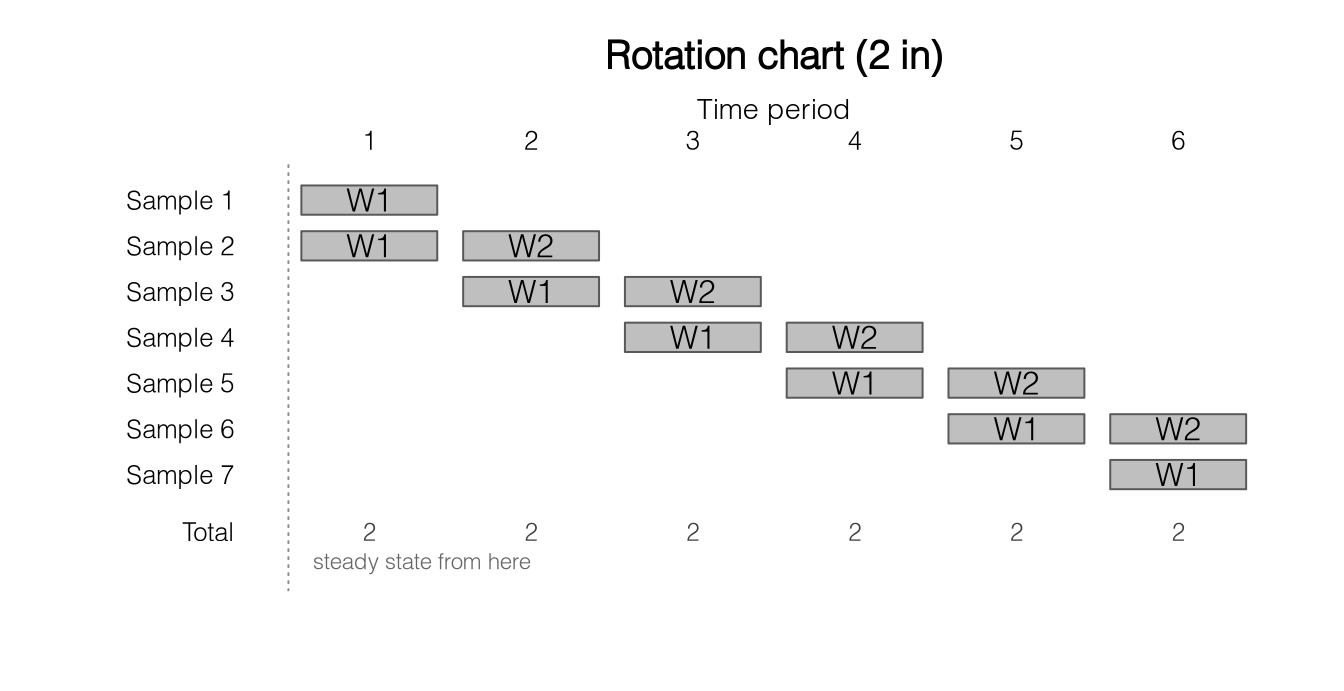
A longitudinal survey observes some units more than once. A rotating panel replaces part of the sample at regular intervals, so it can support both cross-sectional estimates and estimates of change.
This chapter follows one small design from planning to selection. Each cohort is interviewed twice. At a steady state, half of one occasion’s issued sample also appears at the next occasion. The example is deliberately simple and avoids permanent random numbers, unequal-probability sampling, and a choice of longitudinal variance estimator until the basic workflow is clear.
Two packages have different jobs here. svyplan converts precision, response, retention, and overlap assumptions into fieldwork numbers. samplyr selects the start-up and refreshment samples and records which panels are active.
These common designs should not be treated as interchangeable (Smith et al. 2009; Lynn 2012).
| Design | What happens | Basic implementation |
|---|---|---|
| Fixed panel | One sample is interviewed repeatedly | Run execute() once and join later responses to the selected units |
| Fixed panel with entrants | The original panel is kept and new population entrants are added | Draw the original sample and each entrant cohort separately |
| Repeated cross-section | A fresh population sample is drawn on every occasion | Reuse the design with a new frame and seed |
| Rotating panel | Several cohorts are live and one is replaced regularly | Use a start-up partition, then draw one refreshment cohort per occasion |
| Split panel | A continuing panel and a fresh cross-section run together | Keep the two samples and their estimators distinct |
Before choosing among them, state the target population. A fixed wave-1 population cannot represent later births. A cross-sectional target at each occasion needs refreshed frame coverage. samplyr cannot infer that choice from the data.
design_rotation() describes the time a cohort spends in and out of sample. The string "2" means that a cohort is interviewed on two consecutive occasions and then leaves, and design_overlap() reports the overlap it produces.
library(samplyr)
library(svyplan)
library(dplyr)
rotation <- design_rotation("2")
overlap_plan <- design_overlap(rotation)
overlap_plan[1]
#> [1] 0.5
plot(overlap_plan, type = "schedule", start = "immediate")
This is issued-sample overlap. Below full response, the overlap among respondents may differ because response can persist across occasions.
Next, define the responding sample needed for a proportion and allow for response at recruitment and retention into the second interview.
precision_target <- n_prop(p = 0.5, moe = 0.08)

panel_plan <- n_panel(
  precision_target,
  retention = 0.90,
  resp_rate = 0.80,
  design = "rotating",
  start = "immediate"
)

panel_plan
#> Panel recruitment (rotating, 2-wave life)
#> entrants: 99 per occasion -> 150 responding, pooled over 2 cohorts, short of the 151 the target needs
#> proportion (wald): se = 0.04082, moe = 0.08, cv = 0.0816
#>
#>  wave retention n_resp se      moe
#>  1              79     0.05626 0.1103
#>  2    0.9       71     0.05931 0.1162
#>
#> # summary() for the launch, the loss and per-wave cv

fieldwork_plan <- design_schedule(
  panel_plan,
  rotation,
  horizon = 3,
  horizon_policy = "continuing",
  refreshment = "entrant_register",
  rounding = "ceiling"
)
The printed plan reads from the top. The entrants line gives the intake per occasion, 99 after rounding, and the respondents the two cohorts present at an occasion yield together. At a response rate of 0.80 and a retention of 0.90, 99 entrants give about 79 first-interview and 71 second-interview respondents, 150 in all. That is one short of the 151 whole respondents the precision target rounds up to, although 150.5 expected respondents already reach the margin of 0.08. The next line states that target for a proportion near 0.5. The wave table shows each interview alone: 79 and 71 respondents give margins of about 0.11 and 0.12, so the target holds only for estimates pooled over the two cohorts.
The two numbers needed for selection are explicit in the result.
intake_n <- ceiling(panel_plan$n_entrants)

selection_sizes <- c(
  startup = panel_plan$n_cohorts * intake_n,
  intake_each_occasion = intake_n
)
selection_sizes
#>              startup intake_each_occasion
#>                  198                   99
startup is the number issued across the two panels present at the first occasion. intake_each_occasion is the fresh cohort added later. They are not two names for the same sample size.
n_panel() uses the response and retention rates supplied by the planner. It does not estimate attrition, adjust weights for nonresponse, or guarantee that every realized occasion reaches the target. Its optional assurance argument can add a probability-of-reaching-target calculation when that is needed.
The immediate start contains two panels recruited together at occasion 1, and both are then at their first interview. One panel is recruited into a two-interview life and is active on occasions 1 and 2. The other is recruited into a one-interview life and is active only on occasion 1. They differ in life length, not in how far they have already progressed through the retention chain.
data(ken_enterprises)

base_design <- sampling_design() |>
  draw(n = selection_sizes[["startup"]])

startup <- execute(
  base_design,
  ken_enterprises,
  seed = 7,
  panels = fieldwork_plan
)

count(startup, .panel)
#> # A tibble: 2 × 2
#>   .panel     n
#>    <int> <int>
#> 1      1    99
#> 2      2    99
Passing the plan here lets samplyr extract the startup panels and freeze their full activity schedule when the sample is drawn. The partition does not draw future entrants or create later frame vintages. It only organizes this one executed sample.
Materialize an occasion from the recorded schedule with execute(wave = ).
startup_wave_1 <- execute(startup, wave = 1)
startup_wave_2 <- execute(startup, wave = 2)

c(
  wave_1 = nrow(startup_wave_1),
  wave_2 = nrow(startup_wave_2)
)
#> wave_1 wave_2
#>    198     99
Wave activation is a probability subsample, not a row filter. The resulting object carries an activation factor in its weight and can be exported as a two-phase survey design.
class(as_svydesign(startup_wave_2))
#> [1] "twophase2"     "survey.design"
Certainty units and permanent small pools do not follow the overlap declared by this automatic route, so it refuses them. They can still use an explicit data-frame panel schedule when their operational and inference treatment has been decided. Unequal-probability and multi-stage designs also need care in variance estimation. as_svydesign() refuses unsupported combinations rather than silently replacing their variance estimator.
At occasion 2, the start-up panel with a one-interview life has left and a fresh cohort enters. For a dynamic population, that cohort should be drawn from the frame vintage and eligibility definition specified by the survey design.
The synthetic example below creates a separate entrant register. Its distinct identifiers make the cohort frames disjoint by construction.
set.seed(99)

entrants <- ken_enterprises |>
  slice_sample(n = 500, replace = TRUE) |>
  mutate(
    enterprise_id = paste0("NEW_", sprintf("%04d", row_number()))
  )

intake_design <- sampling_design() |>
  draw(n = selection_sizes[["intake_each_occasion"]])

intake_2 <- execute(intake_design, entrants, seed = 8)
rotation_program() records how separately executed cohorts fit into one fieldwork program.
program <- rotation_program(
  cohorts = list(startup = startup, intake_2 = intake_2),
  schedule = fieldwork_plan,
  through = 2
)

occasion_2 <- execute(program, wave = 2)
occasion_2
#> ── Rotation Wave 2 ──────────────────────────────────────────────
#>
#> • startup: 99 rows, panel 1
#> • intake_2: 99 rows, panel 1
#> ℹ Weights are valid within a cohort and are not combined.
The result is a collection with one component per live cohort. It is not automatically row-bound and its weights are not combined. The correct combined estimator depends on who was eligible for each cohort. Disjoint entrant frames are simpler. Refreshment draws from the whole population can give a unit more than one chance of selection and require a union-probability or multiple-frame estimator.
For a longer run, increase horizon when creating fieldwork_plan, repeat the intake step once per occasion, and register the cohorts through the latest fielded occasion. ceiling(panel_plan$n_entrants) is the steady-state intake for each draw.
svyplan::design_overlap() reports overlap from the planned rotation. samplyr::joint_expectation() reports what an executed master records, including block-size remainders. For manually scheduled designs, it also handles permanent certainty units.
executed_overlap <- joint_expectation(startup, waves = c(1, 2))

c(
  planned = overlap_plan[1],
  executed = sum(executed_overlap$take_both) / sum(executed_overlap$take_1))
#>  planned executed
#>      0.5      0.5
Be explicit about the denominator when wave sizes differ. Also say whether the overlap counts issued units or respondents. samplyr knows the first, but response data are needed for the second.
A tbl_sample records selection. Later responses can be joined one-to-one by a stable unit identifier while the sample remains one row per selected unit. Duplicating a selected row once per interview and exporting that long table as a new survey design would count the unit as though it had been sampled more than once.
For two waves derived from the same master, stack_waves() checks their common origin and returns a long table for a longitudinal analysis package.
The establishment frame and the observations below are synthetic. Each occasion supplies a new measurement for every issued establishment. Retain the frame’s baseline revenue under another name, and join the occasion’s interview by enterprise_id. The join preserves the issued rows.
set.seed(101)
interviews_1 <- startup_wave_1 |>
  as.data.frame() |>
  mutate(enterprise_id,
         revenue_millions = revenue_millions * exp(rnorm(n(), 0, 0.1)),
         .keep = "none")
interviews_2 <- startup_wave_2 |>
  as.data.frame() |>
  mutate(enterprise_id,
         revenue_millions = revenue_millions * exp(rnorm(n(), 0.05, 0.1)),
         .keep = "none")

observed_wave_1 <- startup_wave_1 |>
  rename(revenue_baseline = revenue_millions) |>
  left_join(interviews_1, by = "enterprise_id", relationship = "one-to-one")
observed_wave_2 <- startup_wave_2 |>
  rename(revenue_baseline = revenue_millions) |>
  left_join(interviews_2, by = "enterprise_id", relationship = "one-to-one")

survey::svytotal(~revenue_millions, as_svydesign(observed_wave_1))
#>                    total     SE
#> revenue_millions 1121562 232656
survey::svytotal(~revenue_millions, as_svydesign(observed_wave_2))
#>                    total     SE
#> revenue_millions 1136540 377223

wave_table <- stack_waves(observed_wave_1, observed_wave_2)
wave_table |>
  select(wave, master_id, enterprise_id, revenue_millions, design_weight) |>
  head(4)
#> # A tibble: 4 × 5
#>    wave master_id enterprise_id revenue_millions design_weight
#>   <int>     <int> <chr>                    <dbl>         <dbl>
#> 1     1         1 KEN_07583                19.2           85.9
#> 2     1         2 KEN_04572                67.0           85.9
#> 3     1         3 KEN_15975                44.4           85.9
#> 4     1         4 KEN_10870                 6.95          85.9
Both exports use the current occasion’s revenue, including where the retained master carries a same-named baseline column. A missing current measurement would remain missing. It would not fall back to the baseline. The master and the other occasion remain unchanged.
These are separate estimates for the start-up cohort’s frame. The second does not include the refreshment cohort or estimate a growing population’s total automatically. This example assumes complete response on both occasions.
design_weight is the design weight, including activation. It is not a final nonresponse-adjusted or calibrated weight. master_id links the same selected unit across these waves. It is not a cluster identifier.
Two separate cross-sectional variance estimates do not contain the covariance needed for a variance of change. The appropriate longitudinal estimator depends on the design, response process, calibration, and available joint inclusion information. stack_waves() validates the handoff but deliberately does not choose that estimator.
Field substitution, replacing a nonresponding unit with a neighbor, changes the design in a way no weight records. A planned reserve does the same job inside the design. Draw the issued sample together with its reserve, partition it into panels, and declare a release schedule: the first release opens the main panels, and a second, if response falls short, opens the reserve as well.
release <- data.frame(
  panel = rep(1:5, times = 2),
  wave = rep(1:2, each = 5),
  active = c(TRUE, TRUE, TRUE, TRUE, FALSE, TRUE, TRUE, TRUE, TRUE, TRUE)
)
reserve_master <- sampling_design() |>
  stratify_by(region, alloc = "proportional") |>
  draw(n = 250) |>
  execute(bfa_eas, seed = 11, panels = release)

main_release <- execute(reserve_master, wave = 1)
full_release <- execute(reserve_master, wave = 2)
c(issued = nrow(reserve_master), main = nrow(main_release),
  with_reserve = nrow(full_release))
#>       issued         main with_reserve
#>          250          200          250

# The weight factor of the main release, per unit
at <- match(main_release$.sample_id, reserve_master$.sample_id)
range(main_release$.weight / reserve_master$.weight[at])
#> [1] 1.166667 1.500000
Each release is a probability subsample of the issued sample. A unit is released with probability equal to its block’s quota for the released panels over the block size, and its weight is multiplied by the inverse, the block size over that quota. That factor is exact, and it is not the nominal 5/4 when a pool does not divide into full blocks, which is why the range above is not a single value. Releasing the reserve returns every issued unit at its original weight. What a release cannot do is target units: opening the reserve only where response was poor would make the release depend on the outcome, which no weight corrects. Release whole panels, uniformly, and leave the remaining nonresponse to the analysis. ?panel_assignment describes the schedule and its weights.
Permanent random numbers control overlap between separate draws. Panel schedules control how long an already selected cohort remains active. A survey may use both, but neither substitutes for the other. The schedule of this chapter fits a fieldwork rule such as “keep each cohort for two occasions.” The PRNs of Chapter 11 fit a rule such as “make the next draw share more or fewer units with the current draw.”
design_rotation() to describe the cohort life.n_panel() to obtain n_entrants and n_cohorts.panels.execute(wave = ).rotation_program().