ea_register <- bfa_eas |>
  mutate(
    region,
    commune_id = paste(region, province, commune, sep = "/"),
    ea_id,
    ea_households = households,
    .keep = "none"
  )

commune_register <- ea_register |>
  summarise(commune_households = sum(ea_households),
            .by = c(region, commune_id))

head(commune_register, 3)
#> # A tibble: 3 × 3
#>   region            commune_id                 commune_households
#>   <fct>             <chr>                                   <int>
#> 1 Boucle du Mouhoun Boucle du Mouhoun/Bale/Ba…               5089
#> 2 Boucle du Mouhoun Boucle du Mouhoun/Bale/Ba…               2586
#> 3 Boucle du Mouhoun Boucle du Mouhoun/Bale/Bo… 585710 A three-stage household survey
add_stage() starts another selection within each selected parent. This chapter selects communes within regions, enumeration areas (EAs) within those communes, and households within those EAs. The first two stages use PPS without replacement and the last uses simple random sampling without replacement. Selection pauses while the household listing is prepared, then continues under the same design.
bfa_eas is a derived Burkina Faso frame. Its modeled EAs, household counts and historical administrative labels are teaching inputs, not a current official household register. The household listing and interview outcomes below are synthetic.
10.1 Give each register its own sampling unit and size
| Register | One row represents | Key | Measure of size |
|---|---|---|---|
commune_register |
A commune | commune_id, qualified by geography |
Sum of EA household counts in that commune |
ea_register |
An EA | ea_id, with its parent commune_id |
That EA’s modeled household count |
household_listing |
A household in a selected EA | ea_id and local hh_id |
None, equal-probability sampling |
The measure of size belongs to the unit being selected. In one shared hierarchy frame, a commune’s total would have to repeat on each of its EA rows. Separate registers make the two levels explicit. Their order in execute() maps them to stages, and names on a list are labels, not a join specification.
10.2 Declare all three stages
household_design <- sampling_design("Three-stage household survey") |>
  add_stage("Communes") |>
    stratify_by(region) |>
    cluster_by(commune_id) |>
    draw(n = 4, method = "pps_brewer", mos = commune_households) |>
  add_stage("EAs") |>
    cluster_by(ea_id) |>
    draw(n = 3, method = "pps_brewer", mos = ea_households) |>
  add_stage("Households") |>
    draw(n = 12)

household_design
#> ── Sampling Design: Three-stage household survey ────────────────
#>
#> ℹ 3 stages
#>
#> ── Stage 1: Communes ────────────────────────────────────────────
#> • Strata: region
#> • Cluster: commune_id
#> • Draw: n = 4 (per stratum), method = pps_brewer, mos = commune_households
#>
#> ── Stage 2: EAs ─────────────────────────────────────────────────
#> • Cluster: ea_id
#> • Draw: n = 3 (per commune_id), method = pps_brewer, mos = ea_households
#>
#> ── Stage 3: Households ──────────────────────────────────────────
#> • Draw: n = 12 (per ea_id), method = srswor
The takes are four communes per region, three EAs per selected commune, and twelve households per selected EA. The first stage has no allocation rule, so n = 4 is per stratum. A pool smaller than its take is a census, which execution reports. Region stratification does not carry over as a stratum specification to later stages.
10.3 Select areas, then pause for listing
selected_eas <- execute(
  household_design,
  list(commune_register, ea_register),
  stages = 1:2,
  seed = 91
)

selected_eas |>
  as.data.frame() |>
  count(region, name = "selected_eas")
#>               region selected_eas
#> 1  Boucle du Mouhoun           12
#> 2           Cascades           12
#> 3             Centre           12
#> 4         Centre-Est           12
#> 5        Centre-Nord           12
#> 6       Centre-Ouest           12
#> 7         Centre-Sud           12
#> 8                Est           12
#> 9      Hauts-Bassins           12
#> 10              Nord           12
#> 11   Plateau-Central           12
#> 12             Sahel           12
#> 13         Sud-Ouest           12
The EA register covers all communes, and execution restricts it to the selected parents. The result holds the two completed stages and their weights, and it is the starting point for continuation.
selected_communes <- bfa_eas |>
  distinct(region, province, commune) |>
  filter(paste(region, province, commune, sep = "/") %in%
           selected_eas$commune_id) |>
  mutate(status = "Selected commune")

map_eas(selected_eas, outline = "communes", top = "regions",
        fill_data = selected_communes, fill = "status", size = 1.2) +
  labs(fill = NULL)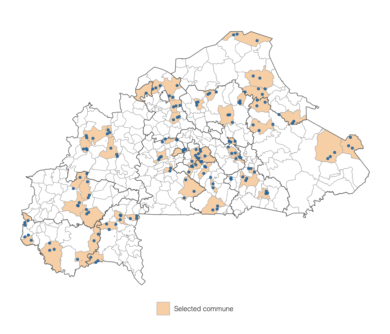
Stratifying the first stage by region spreads the communes over the whole country. The second stage then concentrates the EAs inside those communes, which is what keeps the travel of each field team manageable.
first_commune <- selected_eas$commune_id[1]
commune_eas <- ea_register$ea_id[ea_register$commune_id == first_commune]

map_zoom(commune_eas, selected_eas$ea_id) +
  labs(title = first_commune)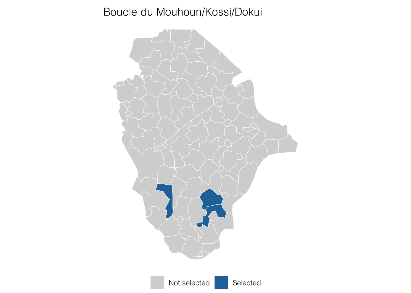
Here the EA stage kept three of the commune’s 115 EAs, each with probability proportional to its modeled household count.
In fieldwork, a listing team enumerates households in the selected EAs. Here an artificial listing gives each selected EA as many households as its modeled count. It creates identifiers, not household records.
household_listing <- selected_eas |>
  as.data.frame() |>
  reframe(hh_id = seq_len(ea_households), .by = c(commune_id, ea_id))

stopifnot(!anyDuplicated(household_listing[c("ea_id", "hh_id")]))
head(household_listing, 3)
#>                      commune_id ea_id hh_id
#> 1 Boucle du Mouhoun/Kossi/Dokui 41769     1
#> 2 Boucle du Mouhoun/Kossi/Dokui 41769     2
#> 3 Boucle du Mouhoun/Kossi/Dokui 41769     3
The listing is a plain data frame because it enumerates candidates for the next stage. The parent EA tells apart household IDs that repeat across EAs.
A real listing rarely finds exactly the number of households the EA was selected on. That does not bias the weights. The EA stage used the measure of size in its register, and the household stage uses the take over the listed count, so each factor is the probability of the selection actually made. What the difference costs is self-weighting. The final weight varies with the ratio of listed to modeled households, and an EA listed with fewer households than the take is taken whole, which execution reports.
When a selected EA is too large to list, it is divided into segments, the segments are counted, and one is selected with probability proportional to its count. That is one more stage between EAs and households, add_stage("Segments") |> cluster_by(segment_id) |> draw(n = 1, method = "pps_brewer", mos = segment_households), with a segment register as its frame. Its probability enters the weight like any other stage’s, and the household listing then covers the selected segment only.
10.4 Continue from the listing
issued <- execute(selected_eas, household_listing, seed = 92)
#> Warning: Stage 3: sample size exceeded the pool population in 3 of 156
#> pools.
#> ✖ Requested 1872 units, selected 1859.
#> ℹ Capped pools: "Boucle du Mouhoun/Kossi/Nouna > 33237",
#>   "Est/Tapoa/Kantchari > 31552", and "Sahel/Oudalan/Tin-Akoff >
#>   34718".
#> ℹ Inspect with `frame_summary(sample, detail = "pool")` and the
#>   capped column.

issued |>
  as.data.frame() |>
  select(commune_id, ea_id, hh_id, .weight_1, .weight_2, .weight_3, .weight) |>
  head(4)
#>                      commune_id ea_id hh_id .weight_1 .weight_2
#> 1 Boucle du Mouhoun/Kossi/Dokui 41769    66  11.85575  24.46053
#> 2 Boucle du Mouhoun/Kossi/Dokui 41769    55  11.85575  24.46053
#> 3 Boucle du Mouhoun/Kossi/Dokui 41769    10  11.85575  24.46053
#> 4 Boucle du Mouhoun/Kossi/Dokui 41769    13  11.85575  24.46053
#>   .weight_3  .weight
#> 1  6.333333 1836.653
#> 2  6.333333 1836.653
#> 3  6.333333 1836.653
#> 4  6.333333 1836.653

stopifnot(isTRUE(all.equal(
  issued$.weight,
  issued$.weight_1 * issued$.weight_2 * issued$.weight_3
)))
frame_summary(issued)
#> # A tibble: 3 × 12
#>   stage unit_level scope    chance_kind     probabilities storage
#>   <int> <chr>      <chr>    <chr>           <chr>         <chr>
#> 1     1 cluster    universe inclusion_prob… exact         units
#> 2     2 cluster    eligible inclusion_prob… exact         units
#> 3     3 element    eligible inclusion_prob… exact         consta…
#> # ℹ 6 more variables: n_pools <int>, N <dbl>, n_target <dbl>,
#> #   n_expected <dbl>, n_realized <dbl>, take_rate <dbl>
The final weight is the reciprocal of the product of the three conditional selection probabilities. Continuation keeps the earlier factors, whereas starting a new design on selected_eas would declare a new sampling phase. The two seeds specify separate reproducible randomization steps, so matching a one-call execution exactly would need the same uninterrupted RNG stream.
A person stage continues the same way from a household roster, for example add_stage("Person") |> draw(n = 1, on_empty = "silent") for one eligible person per household. A selected household with no eligible member has no roster rows. By default that refuses the stage, because a missing roster is more often an error than an empty household. on_empty = "silent" or "warn" accepts such households: they stay in the design, contribute zero to every total, and are counted by summary(). An EA in which no household has an eligible member is left with no row at all. as_svydesign() then warns (samplyr_warning_export_empty_parent), because survey computes that EA’s term within its commune without it, and RWYB refuses the sample. A commune left with no row is refused by every export route.
10.5 Set a household take per EA before selection
The household stage above takes twelve households in every EA. A take that differs by EA and is fixed before any selection is a table keyed by ea_id. Stratifying the household stage by that identifier applies each row within its own EA. The table can cover every EA in the register, although only the selected ones will be listed.
takes <- ea_register |>
  mutate(
    ea_id,
    # Never more than the EA's modeled count.
    n = pmin(if_else(ea_households < 150, 8, 12), ea_households),
    .keep = "none"
  )

per_ea_design <- sampling_design("Three-stage survey, take per EA") |>
  add_stage("Communes") |>
    stratify_by(region) |>
    cluster_by(commune_id) |>
    draw(n = 4, method = "pps_brewer", mos = commune_households) |>
  add_stage("EAs") |>
    cluster_by(ea_id) |>
    draw(n = 3, method = "pps_brewer", mos = ea_households) |>
  add_stage("Households") |>
    stratify_by(ea_id) |>
    draw(n = takes)

areas <- execute(
  per_ea_design,
  list(commune_register, ea_register),
  stages = 1:2,
  seed = 91
)
area_listing <- areas |>
  as.data.frame() |>
  reframe(hh_id = seq_len(ea_households), .by = c(commune_id, ea_id))

per_ea <- execute(areas, area_listing, seed = 92)
per_ea |>
  as.data.frame() |>
  count(ea_id, name = "households") |>
  left_join(takes, by = "ea_id") |>
  head(4)
#>   ea_id households  n
#> 1   674         12 12
#> 2   682         12 12
#> 3   683         12 12
#> 4  1219          8  8
Each selected EA takes its own row, and the rows for EAs that were not selected are simply unused. A mistyped ea_id that matches no selected EA is therefore not caught at this point. Check the table against the register before selection, for example with setdiff(takes$ea_id, ea_register$ea_id).
10.6 Join observations and hand off to analysis
Every issued household responds in this example. The artificial consumption values stand for an outcome collected in the field.
set.seed(93)
interviews <- issued |>
  as.data.frame() |>
  mutate(ea_id, hh_id,
         consumption = round(rlnorm(n(), log(100000), 0.5)),
         .keep = "none")

observed <- issued |>
  left_join(interviews, by = c("ea_id", "hh_id"), relationship = "one-to-one")
stopifnot(nrow(observed) == nrow(issued))
With real nonresponse, keep the issued rows and join response indicators and measurements to them. Sampling weights describe selection, and dropping nonrespondents is not a response adjustment. The analyst chooses and justifies that adjustment downstream.
linearized <- as_svydesign(observed)
survey::svymean(~consumption, linearized)
#>               mean     SE
#> consumption 113266 1529.6
This export uses Brewer’s variance approximation for the PPS stages. Exact first-order probabilities do not make that variance approximation exact. svrep’s RWYB replicates are an alternative, also approximate for PPS without replacement.
set.seed(94)
replicated <- as_svrepdesign(observed, type = "rwyb", replicates = 500)
#> Warning: RWYB uses an approximation for unequal-probability sampling
#> without replacement.
#> ℹ It does not reproduce the sampler's exact joint inclusion
#>   probabilities.
survey::svymean(~consumption, replicated)
#>               mean     SE
#> consumption 113266 1485.8
The warning describes the PPS approximation. More replicates reduce simulation error, not the error of the variance approximation. Designs that need more than this handoff, such as two phases, joint inclusion probabilities and overlapping frames, are the subject of Chapter 13.